nanosims-wiki

2017-11-04:

In addition to nanoSIMS images, I have imaged the same field of view (FOV) also with another instrument (e.g., fluorescence microscope, AFM, SEM, TEM). I would like to analyze the nanosims and external image data together in LANS. Specifically, I would like to align them, overlay them, extract lateral profiles, define ROIs based on the external image, calculate ion count ratios in these ROIs, plot scatter plots of nanosims vs. external data, etc.

1. There is a new menu item External in the main LANS GUI for aligning, importing and performing combined analysis of the external and nanosims image data.
2. After importing, the data from the external image behave within LANS as an additional mass called ext. This means that you can use it as such in LANS processing actions.

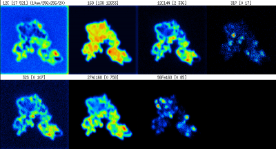
Here we will describe, by means of an example, how to work in LANS with an external image data generated by AFM. We will use unpublished data kindly provided by Lydia Pohl, TU Munich, and assume that the nanosims images look like this

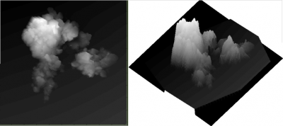
while the external data look like this

Specifically, we will describe how to

1. Align the external and nanosims images
2. Import the aligned external image to LANS
3. Combine the data from the external and nanosims images in order to
   • Display a 3D overlay between the external and nanosims images (ion counts or ratios)
   • Define ROIs based on the external image
   • Display scatter plots of nanosims vs external data
   • Display lateral profiles overlays

1. If required, use an image manipulation program of your choice to make corrections to your external image. For example, you could correct for the uneven background, rotate or vertically/horizontally flip the image so that it looks more similar to the ion counts images shown by LANS, etc. After performing such corrections, save the image as a gray-scale bitmap image, preferably as TIF, BMP or PNG. You can skip this point if you do not wish to make any corrections.
2. Select Align external and nanoSIMS images from the External menu in LANS. This will open a new window with a dedicated GUI that will enable you to make a more accurate alignment between the external and nanoSIMS images.
3. In this window select File → Load external image from the menu, and select the file with your external image data. Note that several binary and text-based input formats are supported. The default is TIF, but alternatives include BMP or PNG. In this example the external image represents the height of a surfacet (in meters) obtained by AFM. Therefore, we will import it as XYZ. This format is a standard format available from AFM instruments, and consists of three columns of data representing the x, y and z coordinates of the scanned surface. After you select it, the XYZ data is processed, and in a window that pops up you are asked to provide input for rescaling the external image. Normally, at this point, you should not need to change the x-size or y-size of the external data, as these are derived automatically, but you should verify that the suggested values are correct. In contrast, you can modify the value for the z-scale conversion factor. If the z-data in your XYZ file are in meters (as they are now) and you would like to show them later on in nano-meters, you should enter in the Conversion factor for z-data field the value of 1.0e9 (as suggested by default).
4. Select File → Load nanosims image from the menu, and select one of the nanoSIMS images that you produced while analyzing your nanoSIMS data. The best choice is one of the *.mat files, which you can find in the mat folder as a result of your previous processing of the nanoSIMS data. Note that this image should be chosen such that it best resembles the external image. In this way a good alignment, which you are going to work on next, will be possible. After these steps, the alignment GUI should look similar to this one.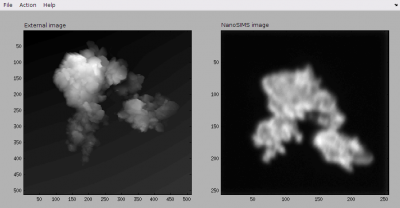
5. Now you are ready to work on the alignment of the two images. This is done through the Action menu. First, add a point in the external image and immediately afterwards add a corresponding (matching) point in the nanosims image. Repeat this until you defined at least four such corresponding (matching) point pairs. Use your best intuition to produce these point pairs. Note that at any time you can modify a point's location. When doing so, note the hints displayed in the Matlab console, as these are very useful for you to figure out how to select and move points around the image using a mouse or arrow keys. After some effort, the GUI with the external and nanoSIMS images together with the corresponding point pairs should look similar to this one.
6. Save the locations of the point pairs using the File → Save point list menu. This may be useful if you need to modify the location of any point in the future.
7. If you think your definition of the point pairs is correct, select Action → Calculate and show the alignment. If you want to apply some extra fine tuning to the external image, specify the respective parameters in the dialog window that pops up. Normally, you will not need to do this, so simply click OK. Immediatelly afterwards you will be presented with an overlay between your external (in red) and nanosims (in green) images, calculated based on the point pairs that you have defined until this point.
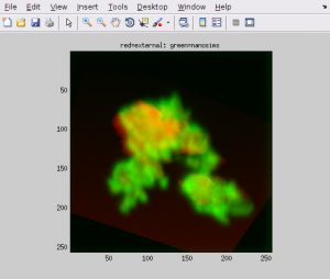
8. If you are not satisfied with the alignment result, try to modify the locations of the points that you have defined already, or try to add more points. The latter option may help you force the stretching of the external image such that it better matches the nanosims image.
9. If you are satisfied with the alignment result, you need to export it. To do this, use Action → Export aligned external image from the menu, and specify the folder and filename of the output. In this example, we will save the output in the mat folder under the filename AFM_aligned.mat. By selecting the *.mat output format we specify that we do care about the actual values in the external image. Clearly, this is because in our case the values correspond to the height of the surface in nano-meters.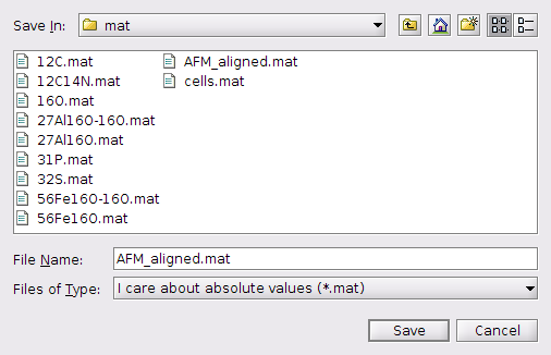
10. After these steps the first stage is finished and you can close the GUI for the image alignment.

1. To import the aligned external image to LANS, use External → Select aligned external image from the main LANS menu. Change the file type to MAT files (*.mat) and select the file created in the first stage (in this example the file AFM_aligned.mat). Read the message that pops up and click OK.
2. If you have read the message carefully, you will now know that from this point onwards the data from the imported external image will behave within LANS as an additional mass called ext. This means that you can use it as such in LANS processing actions, such as for defining ROIs, calculating ratios, displaying lateral profiles or scatter plot, etc. (see below).
3. If you want to stop using the external image, you need to clear its content. Do this by selecting External → Select aligned external image and pressing cancel when prompted for the external image file in the file selection dialog that pops up. Again, a message should pop up, this time notifying you that the external image is no longer available.

Knowing that the imported external image behaves in LANS as any other mass image (secondary ion counts image), you can make a number of analyses where the data from the external image is combined with the nanosims data. Here are a few examples.

1. Select External → 3D overlay masses with external image from the main LANS menu. The follwing GUI window will pop up.
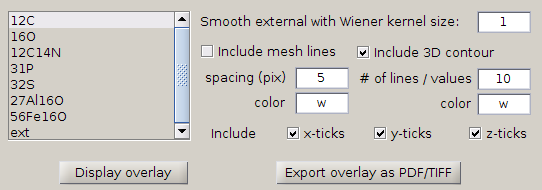
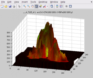
2. In this window, select one or more masses that you want to overlay with the external image and click on Display overlay. Depending on whether you do or do not include the mesh lines, 3D contour, etc., you will get something similar to one of the views shown below. Specifically, the color-coded values of the secondary ion counts are superimposed onto the surface defined by the AFM data. Note that in this example the z-scale is nano-meters (height of the surface), while the color scale of the secondary ion counts is defined by the values in the corresponding scale fields in the main LANS GUI. If you want to change this scaling you need to close the 3D overlay GUI, change the scale, and repeat point 1.
3. Use the 3D rotate tool available in the toolbar of the figure to ratate the view of the displayed overlay. When you like it, you can export it by clicking Export overlay as PDF/TIFF.
4. Select External → 3D overlay ratios with external image from the main LANS menu. A GUI window similar to the one shown above will pop up, but this time with ratios instead of masses.
5. In this window, select one or more ratios that you want to overlay with the external image and click on Display overlay. Again, depending on selected options, you will get something similar to the view shown below, which you can rotate and export as you wish.

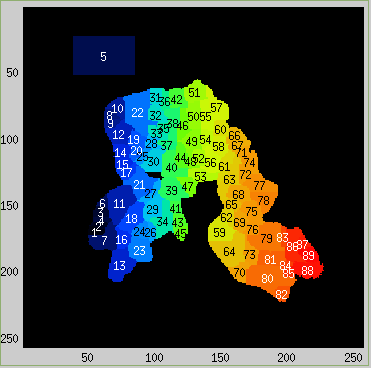
1. Type ext in the ROI definition template text field in the main LANS GUI.
2. Select ROIs → INTERACTIVE ROIs definition tool from the main LANS menu. This will make it possible to define ROIs based on data in the external image.

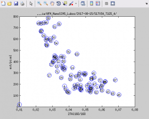
One way to identify the relationship between the data in the external image and the nanosims data is by plotting a scatter plot of values averaged over ROIs. In this example, we will check for a relationship between the ratio 27Al16O/16O and the surface height (derived from the data in the external AFM image) in ROIs that look as shown below. All steps are done through the main LANS GUI.

1. In the first text field for the ratio expressions (see image below), type the expression of your choice (e.g., 27Al16O/16O).
2. In the second text field for the ratio expressions, type the expression ext/pixel. The reason to normalize the values in the external image by pixels is to make it possible to calculate for each ROI the average height of the pixels in the ROI. Note that this normalization is quite essential, as without it the displayed values would be the height accumulated over all pixels in the ROI, which is obviously not what we want to study in this example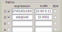
3. Type 1 and 2 in the R/x and G/y fields in the main LANS GUI, check the Plot x-y-z graph checkbox, and select Output → Display ratios from the main LANS menu. You will obtain a scatter plot similar to this one.

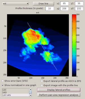
Another way to identify the relationship between the data in the external image and the nanosims data is by overlaying lateral profiles. In this example, we will check for a relationship between the ion counts 27Al16O and 12C14N and the surface height (derived from the data in the external AFM image).

1. Check Display lateral profiles in the main LANS GUI.
2. Select Output → Display masses from the main LANS menu.
3. In the window that pops up, select ext in the top-left pop-up menu and use the mouse to draw a line along which the lateral profiles will be calculated.
4. Set the profile thickness to something like 10 so that the displayed data will be an average of data points in a band of 10 pixels parallel to the drawn line.
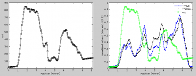
5. Click on Display lateral profiles to display the surface height as a function of distance along the profile (see below, left figure).
6. Check the Show normalized in one graph option, select 27Al16O, 12C14N and ext in the list of masses below this check box, and click on Display lateral profiles. This will draw an overlay between the selected ion counts and the height as a function of the distance along the profile (see below, right figure). Note that in this overlay the values are normalized such that the range defined by the minimum and maximum values for each displayed variable is mapped to 0 and 1, respectively. The minimum and maximum values are taken from the respective scale text fields in the the main LANS GUI.

Back to the list